Introduction

This introduction addresses some of the key concepts of FaIR and how they are now implemented inside the model. For worked examples of FaIR and the energy balance model, take a look at the Examples.

FaIR produces global mean temperature projections from various forcers. Input datasets can be provided in terms of emissions, concentrations (for greenhouse gases), or effective radiative forcing. Different species can be input in different ways, if they are internally consistent and valid (e.g. if you want to provide CO₂ and short-lived climate forcer emissions, with concentrations of non-CO₂ greenhouse gases and prescribed forcing for volcanic and solar forcing, like the esm-hist runs of CMIP6 Earth System Models). You can provide any number of species from single-forcing runs to full climate assessments. In “full-climate” mode, the process diagram in FaIR is similar to Fig. 1.

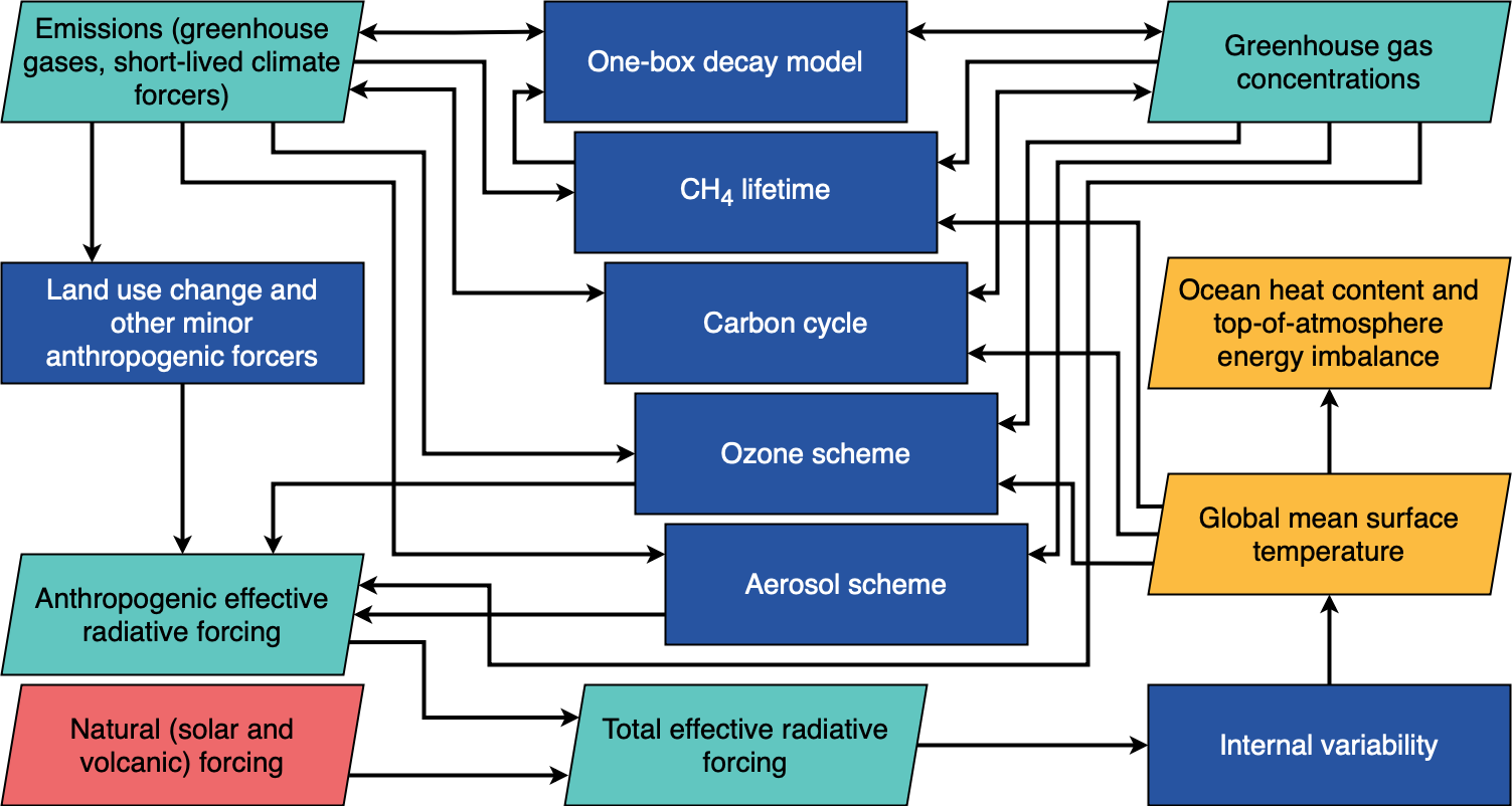
Fig. 1 Simplified outline of available processes in FaIR. Some processes have been omitted for clarity.

FaIR is now a primarily object-oriented interface. The main interaction with FaIR is through the FAIR class instance:

from fair import FAIR
f = FAIR()

FAIR() contains the attributes and methods required to run the model. The energy balance climate model can also be run in standalone mode with prescribed forcing. In the rest of this introduction, f is taken to be a FAIR instance.

Typically there are two stages to a FaIR run. The first is to set up the dimensionality of the problem (define time horizon, included species and how to implement them), and the second is to fill in the data and do the run.

Dimensionality

Internally, variables in are book-kept with numpy arrays that have up to five dimensions:

Not all variables include all dimensions, but they are always in this order.

Parallelisation allows more than one scenario and one set of configs to be run at the same time. time is the only axis which is looped over, allowing high efficiency multiple-scenario or multiple-configuration runs to be done on the same processor (subject to available RAM and disk space).

For inputs and outputs, we use xarray, which wraps the numpy arrays with axis labels and makes model input and output a little more tractable.

Defining the dimensionality of the problem is the first step of setting up FaIR.

Time

FaIR uses two time variables to keep track of state variables: timepoints and timebounds. Only emissions are defined on timepoints, where everything else is on timebounds. As the name suggests, timebounds are on the boundary of model time steps, and timepoints are nominally at the centre of the model time step. Fig. 2 illustrates this.

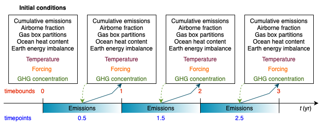
Fig. 2 Timebounds (red) and timepoints (blue) in FaIR, showing associated state variables defined on each time variable. FaIR can be run with prescibed emissions (blue arrows) and/or with prescribed concentrations for greenhouse gases (green arrows).

Time is specified in years, but you are not forced to use integer years. This can be useful for coupling directly with integrated assessment model derived emissions (often 5- or 10-year timesteps) or assessing short-term responses to volcanic forcing, where sub-annual responses can be important. Fig. 3 shows the timestepping for a \(1/4\)-year timestep.

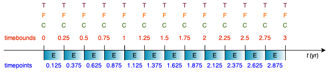
Fig. 3 Timebounds (red) and timepoints (blue) in FaIR using a quarter-year time step.

A FaIR ecosystem therefore contains \(n/{\delta t}\) timepoints and \(n/{\delta t} + 1\) timebounds where \({\delta t}\) is the timestep and \(n\) is the number of years.

Time is defined as so:

f.define_time(start, end, timestep)

You can label time how you wish. Common runs for climate projections will start with a pre-industrial reference year (maybe 1750 or 1850), and run to 2100 or beyond:

f.define_time(1750, 2100, 1)

Or you might want to run an idealised pulse experiment, in which case it’s less informative to assign real years and it is better to start at zero:

f.define_time(0, 1000, 1)

The simple non-integer example from Fig. 3 would thus be:

f.define_time(0, 3, 0.25)

We adopt the pandas practice of including the end point.

For intepreting real dates, the timebound 1750 refers to 00:00 on 1 January 1750, and the timepoint 1750.5 is a mid-year average of the period 00:00 on 1 January 1750 to 00:00 on 1 January 1751. FaIR makes no adjustments for leap years or month length, and assumes each year is 365.24219 days long. The temporal difference between timebound and timepoint can be important when interpreting and reporting results: does temperature in 2100 mean at the timebound 2100, or do we want a mid-year average (corresponding to timepoint 2100.5, in which case we might want to interpolate or take an average of the 2100 and 2101 timebounds.)

Scenarios

A scenario is a set of emissions/concentration/forcing inputs and climate responses. Multiple scenarios can be run in parallel. They are defined as a list of names, for example:

f.define_scenarios(['ssp126', 'ssp245', 'ssp370'])

Note at this stage we are only defining names: no data is being input into FaIR.

Configs

A config defines a set of climate and species parameters to run FaIR with. For example, we might want to run with emulations of a few CMIP6 models, which have different climate sensitivities, aerosol forcing sensitivities to precurors, carbon cycle feedback strengths, and so on:

f.define_configs(['UKESM', 'NorESM', 'GFDL', 'MIROC'])

Again, we are only defining names at this stage.

Combined with the three scenarios above, we have a matrix of 12 runs: each of three emissions scenarios will be run with each of four climate configs.

Species

A specie is anything that forces climate or other species in FaIR, which is a broad definition. This includes greenhouse gases, aerosol precurors, ozone precursors as expected, but also forcing categories (aerosol-radiation interactions, ozone forcing, land-use forcing) that may be calculated from other species.

Each specie has an associated dict of properties which defines how it is implemented in the particular run of FaIR and how it behaves. A properties dict for a CO₂ run might look like:

properties = {
    'CO2': {
        'type': 'co2',
        'input_mode': 'emissions',
        'greenhouse_gas': True,
        'aerosol_chemistry_from_emissions': False,
        'aerosol_chemistry_from_concentration': False,
    }
}

The five dict keys of type, input_mode, greenhouse_gas, aerosol_chemistry_from_emissions and aerosol_chemistry_from_concentration are all required. Both type and input_mode are from pre-defined lists. The API reference for fair.FAIR.define_species explains more.

Species are then declared in FaIR with:

f.define_species(['CO2'], properties)

Basic checks are performed to ensure that input specifications make sense (e.g. you cannot run a type solar in emissions mode, and many species types must be unique). An error will be raised if an invalid combination of options is provided.

For all but single-forcing experiments, defining species this way could be quite onerous. To grab an emissions-driven run using all species known to FaIR with their default values, use:

species, properties = read_properties()
f.define_species(species, properties)

Box and layer

FaIR uses a multiple-box atmospheric decay model with lifetime scaling for greenhouse gases (see e.g. [Millar2017]). This is represented by the box dimension. By default, there are 4 boxes, but this can be modified in the initialisation:

f = FAIR(n_gasboxes=3)

or by accessing the attribute directly after initialisation:

f.n_gasboxes=3

layer refers to the ocean layer of the energy balance model. By default, FaIR uses 3 layers, though this can be modified in the initialisation of the class:

f = FAIR(n_layers=2)

or by accessing the attribute directly:

f.n_layers=3

State variables

State variables are attributes of the FAIR class. All state variables are outputs, and many are valid inputs (particularly for the first timebound in which many must be provided with an initial condition).

After problem setup (see ref:Dimensionality), these xarrays will be created inside FaIR with:

f.allocate()

Dimensions with invalid combinations are retained in the output (e.g. f.emissions will be np.nan for solar forcing) to maintain alignment between datasets.

Emissions

Emissions are the only variable defined on timepoints, and are quantified as an emissions rate per year. FaIR will automatically adjust the emissions flows if a non- annual timestep is provided. Emissions are input or output as the emissions attribute of FAIR:

f.emissions :: [timepoint, scenario, config, specie]

Concentrations

For greenhouse gases, concentrations can be input, or calculated:

f.concentration :: [timebound, scenario, config, specie]

Note the FaIR variable name is concentration, in the singular.

When running in emissions mode, the initial concentration of a greenhouse gas should be specified (at timebound 0). We provide a convenience function, initialise(), for specifying initial conditions:

from fair import initialise
initialise(f.concentration, 278.3, specie='CO2')

You could also directly modify the f.concentration xarray by label:

f.concentration.loc[dict(timebound=1750, specie='CO2')] = 278.3

or position, if you know that CO₂ is index 0 of the specie axis:

f.concentration[0, :, :, 0] = 278.3

Effective radiative forcing

At the per-species level, effective radiative forcing can be input or calculated:

f.forcing :: [timebound, scenario, config, specie]

We use the shorter name forcing, which should be taken to represent effective radiative forcing.

For some species like solar and volcanic, specifying forcing is the only valid input mode.

Again, initial forcing must be provided. In many cases, this will be zero for every species, in which case we don’t have to specify it for each specie:

initialise(f.forcing, 0)

The total effective radiative forcing is an output only:

f.forcing_sum :: [timebound, scenario, config]

and is simply forcing summed over the specie axis.

Units are W m^-2.

Temperature

Temperatures in FaIR are expressed as anomalies (in units of Kelvin) relative to some reference state, usually pre-industrial. Temperature is calculated from an \(n\)-layer ocean energy balance model:

f.temperature :: [timebound, scenario, config, layer]

The temperature near the surface and hence of most importance is layer 0. Again, initial conditions of temperature in all layers should be provided, and for a “cold-start” model can be done with:

initialise(f.temperature, 0)

One of the most important sources of climate projection uncertainty is the temperature response to forcing, which is governed by the climate_config parameters (see later). These are varied across the config dimension in FaIR. Simply, these define how much, and how quickly, temperature change occurs in response to a given forcing and encapsulates ECS and TCR which are emergent parameters.

Airborne emissions

Airborne emissions are the total stock of a specie present in the atmosphere and usually expressed as an anomaly relative to pre-industrial:

f.airborne_emissions :: [timebound, scenario, config, specie]

Again, airborne_emissions should be initialised. For “warm-start” runs, airborne emissions may be non-zero, and this value has influence on the carbon and methane cycles in FaIR.

Airborne fraction

Airborne fraction is the fraction of airborne emissions remaining in the atmosphere:

f.airborne_fraction :: [timebound, scenario, config, specie]

It is simply f.airborne_emissions divided by f.cumulative_emissions. It does not need to be initialised.

Cumulative emissions

The cumulative emissions are the summed emissions since pre-industrial:

f.cumulative_emissions :: [timebound, scenario, config, specie]

cumulative_emissions needs to be initialised. It is used in the carbon cycle and land use forcing components of FaIR.

Ocean heat content

The ocean heat content change is the time integral of the top of atmosphere energy imbalance (after some unit conversion):

f.ocean_heat_content_change :: [timebound, scenario, config]

Units are J. Divide by \(10^{21}\) to get the more common zettajoules (ZJ) unit. It does not need to be initialised.

Stochastic forcing

If using stochastic internal variability, this is the stochastic component of the total effective radiative forcing (see [Cummins2020]). Its dimensionality is:

f.stochastic_forcing :: [timebound, scenario, config]

Units are W m^-2. It does not need to be initialised.

Top of atmosphere energy imbalance

Follows from the energy balance model:

f.toa_imbalance :: [timebound, scenario, config]

Units are W m^-2. It does not need to be initialised.

Gas box partition fractions

The partition fraction is the only state variable where the timebound is not carried, which would necessitate a 5-dimensional array and use up useful memory. So we have:

f.gasbox_fractions :: [scenario, config, specie, gasbox]

Inputting variable data

Once the state variables have been allocated, we need to fill our input variables with data. Any valid method for inputting data into xarray can be used. Additionally, we have a second convenience function fill() that can do this for us:

from fair import fill
fill(f.emissions, 38, specie="CO2", scenario="ssp370")

Browse the Examples for instances where the variables are filled in.

Adjusting configs

For each defined config (in our earlier example, we used the names from four CMIP6 models), we can (and should!) vary the model response. This gives us our climate uncertainty. There are two types: climate_configs and species_configs. As with the state variables, they are attributes of the FAIR instance, and implemented as xarray Datasets.

Climate configs

climate_configs define the behaviour of the energy balance model and contain the following variables:

• ocean_heat_transfer

• ocean_heat_capacity

• deep_ocean_efficacy

• forcing_4co2

• stochastic_run

• sigma_eta

• sigma_xi

• gamma_autocorrelation

• seed

They can be filled in for example using:

fill(f.climate_configs["ocean_heat_capacity"], [2.92, 11.28, 73.25], config='UKESM')

The API reference for the energy_balance_model explains more.

Species configs

species_configs define the behaviour of individual species: most variables have a species dimension, some also have a gasbox dimension. It contains the following variables:

• tropospheric_adjustment

• forcing_efficacy

• forcing_temperature_feedback

• forcing_scale

• partition_fraction

• unperturbed_lifetime

• molecular_weight

• baseline_concentration

• iirf_0

• iirf_airborne

• iirf_uptake

• iirf_temperature

• baseline_emissions

• g0

• g1

• concentration_per_emission

• forcing_reference_concentration

• greenhouse_gas_radiative_efficiency

• contrails_radiative_efficiency

• erfari_radiative_efficiency

• h2o_stratospheric_factor

• lapsi_radiative_efficiency

• land_use_cumulative_emissions_to_forcing

• ozone_radiative_efficiency

• aci_scale

• aci_shape

• cl_atoms

• br_atoms

• fractional_release

• ch4_lifetime_chemical_sensitivity

• lifetime_temperature_sensitivity

There are a lot of things that can be modified here. If you want to use default values for your defined species, you can use:

f.fill_species_configs()

To override a default (or to fill it in if you didn’t use fill_species_configs()), modify the xarray directly or use fill():

fill(f.species_configs["aci_shape"], 0.0370, config='UKESM', specie='Sulfur')

Run

As simple as:

f.run()

The outputs are stored in the xarray attributes. For example, if you ran emissions-driven, you should (if everything worked) find concentrations in f.concentration calculated for species that were declared as greenhouse gases. And vice versa: FaIR will automatically back-calculate emissions where greenhouse gas concentrations are provided, if you set up your run this way.

If you find unexpected NaNs in your outputs, it’s likely that something wasn’t initialised in the above steps. Take a look at the Examples for workflows that should reproduce. If you can’t figure it out and think it should work, raise an issue.

Glossary

ECS

The equilibrium climate sensitivity (ECS) is the long-term equilibrium global mean surface temperature response to a doubling of pre-industrial atmospheric CO₂ concentrations with all other forcers fixed at pre-industrial. It is a measure of long-term sensitivity of climate.

TCR

The transient climate response (TCR) is the global mean surface temperature change at the point where double pre-industrial atmospheric CO₂ concentration is reached in an experiment where CO₂ concentration is increased at a compound rate of 1% per year and all other forcers fixed at pre-industrial. This is around 69.7 years (many models use 70 years). It is a measure of both long-term sensitivity of climate and medium-term rate of climate response.